Using our PivotTables
Production of simple tabulations
The Microsoft Excel file which includes the PivotTable can be opened in the same way as any normal Excel file. When you first open an Excel PivotTable file, you will be presented with a spreadsheet which looks like this:
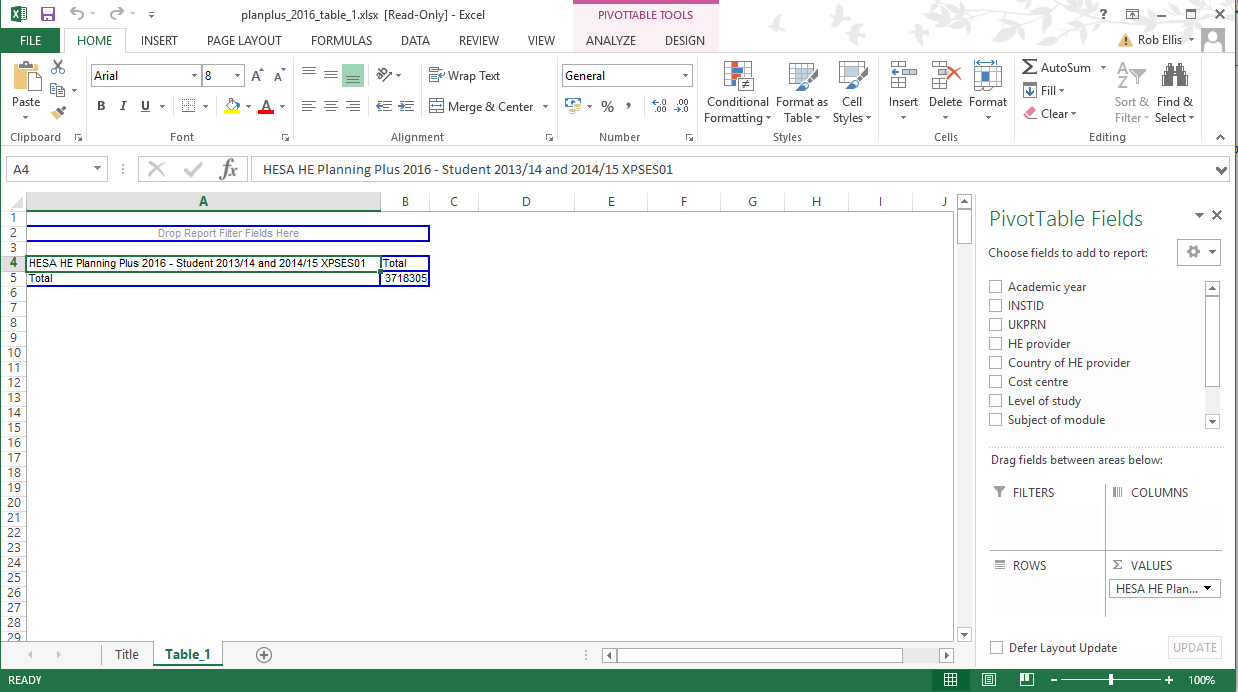
A label such as the one above (“HESA HE Planning Plus 2016 - Students 2013/14 and 2014/15 XPSES01”) will include information about the type of product (in this example HE Planning Plus) as well as information about the academic year of the data.
Only one number will appear. This is the grand total for all the data items held within the data set.
You should note that when the grand total cell is selected, the PivotTable Field List appears on the right (see above).
Now you need to determine the format of the tabulation you want to produce. You can ‘drag and drop’ fields to make columns, rows and filters. You can drag fields and drop them into the cells marked 'total'.
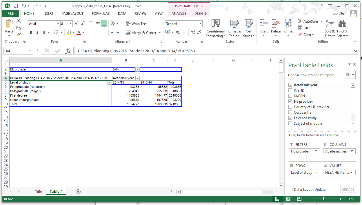
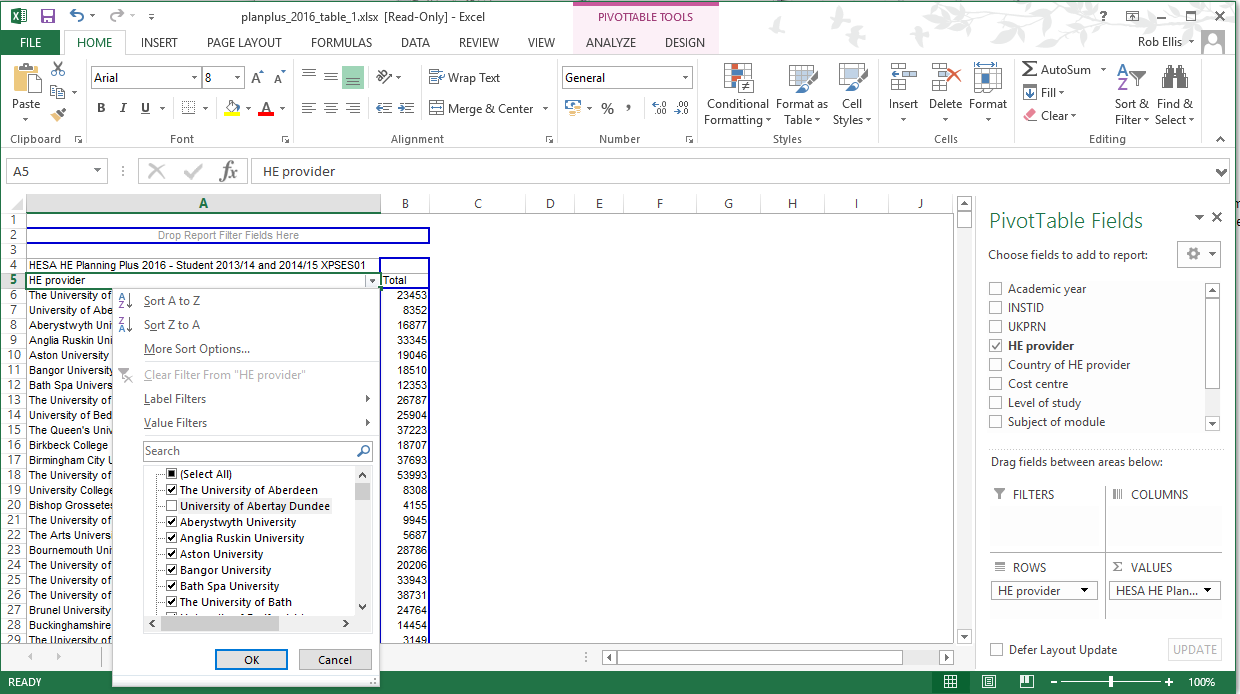
As you can see in this case, we have level of study (rows) tabulated against academic year (columns). We have also placed the field ‘HE provider’ into the filter at the top, but it is not yet active. The down arrow button next to this can be selected to present a menu of the available criteria (in this case a list of institutions). If we check the ‘select multiple items’ box, deselect ‘all’ and select ‘The University of Aberdeen’ and then click ‘OK’ the PivotTable is re-calculated to give the following:

Now all data shown in the table only relates to students at The University of Aberdeen.
You can place more than one field within any of the row, column or page areas of the template. In the following example we have selected Level of study and HE provider as rows by dragging and dropping the HE provider field to the left of the Level of study field:
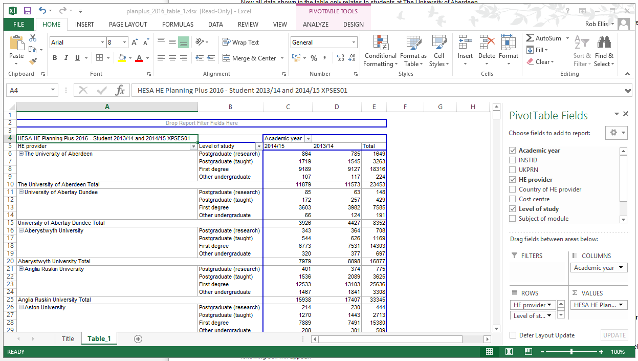
It should be noted that no fields should be placed in the ‘Data’ area as this is pre-loaded when you open the pivot table.
Individual PivotTable fields can be further manipulated by means of the ‘field settings’ option. This can be found by right clicking on the field and selecting ‘field settings’, the following box will appear:
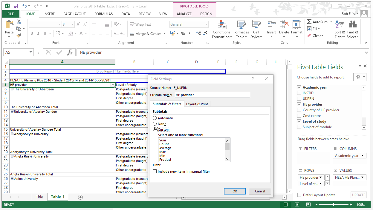
If you then select ‘custom’ this allows you to choose whether you wish totals, subtotals of other arithmetic operations to be performed on the field.
By selecting the drop down arrow next to a field name you can display a list of items and ‘tick boxes’. This gives you the opportunity to hide certain items within the list. In the example below the list of providers contained within the ‘HE provider’ field are displayed. By deselecting the tick box next to the ‘University of Abertay, Dundee’ we can hide this item from the list of providers in the data and exclude it from the grand total. You can do this for as many items as you like.
Grouping data
You may sometimes wish to ‘group together’ existing entries within fields. In the example below, we may wish to generate a postgraduate entry which is a sum of the postgraduate research and postgraduate taught categories. To do this we must use the ‘group’ function.
The first stage is to create a tabulation which only includes the field you wish to group, in this example a level of study tabulation is used.
The second stage is to use the mouse pointer to highlight the categories for grouping. Then right click with the pointer over your selection and click on ‘group’:
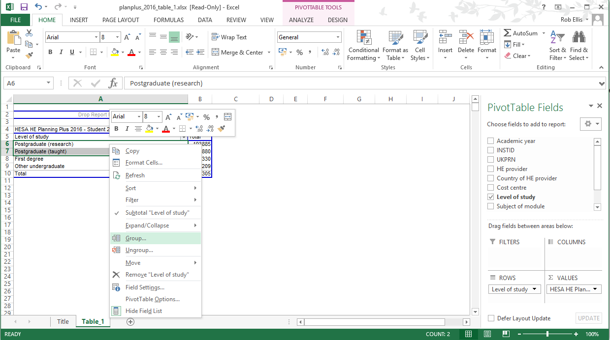
The tabulation then changes, as illustrated in the following diagram:

As you can see, the PivotTable has generated a new user-defined field and by default called it ‘Level of study2’ (though you can rename this with any label you wish). A new entry has been incorporated into the new field and labelled ‘Group1’ (again, by default). As this stage it is a good idea to re-label this new entry by simply over-typing a new name e.g. ‘Postgraduate’. Once this has been done, the new field will appear in the ‘PivotTable Field List’, and can be used like any other existing field.
By right clicking and selecting ‘ungroup’ you can reverse the process above.
Other Pivot functions
There are numerous other PivotTable functions which can be used to manipulate the data including ordering and creation of additional derived data fields. We will not explain these advanced functions in detail here, but guidance on the use of these can be found within the Excel help files.